
| 일 | 월 | 화 | 수 | 목 | 금 | 토 |
|---|---|---|---|---|---|---|
| 1 | ||||||
| 2 | 3 | 4 | 5 | 6 | 7 | 8 |
| 9 | 10 | 11 | 12 | 13 | 14 | 15 |
| 16 | 17 | 18 | 19 | 20 | 21 | 22 |
| 23 | 24 | 25 | 26 | 27 | 28 | 29 |
| 30 |
- Class Incremental
- Energy-based model
- Continual Learning
- mmcv
- Vector Quantized Diffusion Model for Text-to-Image Synthesis
- Facial Landmark Localization
- 베이지안 정리
- learning to prompt for continual learning
- PnP algorithm
- L2P
- Img2pose
- timm
- ENERGY-BASED MODELS FOR CONTINUAL LEARNING
- prompt learning
- CVPR2022
- img2pose: Face Alignment and Detection via 6DoF
- VQ-VAE
- Mask-and-replace diffusion strategy
- Discrete diffusion
- requires_grad
- Mask diffusion
- DualPrompt
- Class Incremental Learning
- state_dict()
- Face Alignment
- learning to prompt
- CIL
- Face Pose Estimation
- Markov transition matrix
- VQ-diffusion
- Today
- Total
Computer Vision , AI
Deep Equilibrium Models (DEQ) 리뷰 본문
Deep equilibrium model에 대한 정리
일반적인 deep neural network를 수식의 형태로 표현해보면 다음과 같이 표현할 수 있을 것이다.

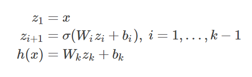
sigma: activation function
W_i: weights of i-th layer
b_i: bias of i-th layer
z_i : latent vector of i-th layer
각 annotation이 다음과 같을 때 i+1번째 layer의 latent vector의 값은 이전인 i번째 latent vector가 W_i를 통과하여 bias b_i를 더해준 뒤 activation function을 거쳐 nonlinearity를 확보한 형태라고 할 수 있을 것이다.


위의 일반적인 neural network를 넘어서 weight-tied, input-injected 형태의 layer를 가진 neural network를 생각해보자.
i-th layer의 weight와 bias를 독립적인 weight와 bias로 하지 않고 하나의 weight W와 bias b를 사용하는 형태이다.
구체적으로 설명하면 i+1번째 layer의 latent vector는 i 번째 latent vector에 전 layer에서 공유하는 weight W를 거쳐 input tensor x에 보조적인 weight U를 거쳐서 나온 결과 (x의 선형변환)와 bias를 더해주고 activation function을 씌운 형태라고 할 수 있다. 놀랍게도 이런 형태의 neural network도 일반적인 neural network과 비교하여 상당히 잘 작동하는 것을 확인할 수 있다.
DEQ에서는 여기서 한가지 가정이 들어간다. 위의 weight-tied, input-injected layer를 무한정 반복한다고 생각해보자, i가 무한대로 된다고 할 때 일반적인 neural network에서는 latent vector가 fixed point 혹은 equilibrium point라고 할 수 있는 z*에 수렴할 것이라는 것이다.


다시 말하면 이 equilibrium equation이 fixed point z*를 output으로 낼 수 있는 근을 찾으면 forward pass를 무한대로 반복하지 않고서도 이를 반복한 것과 같은 효과를 낼 수 있다는게 DEQ의 핵심이다. [Winston and Kolter, 2020] (fixed point의 존재 및 고유 여부에 관한 보장)
여기서 Ux가 필요한 이유가 나오는데 fixed point z*에 대한 식을 보면 Ux가 없으면 input tensor x에 대한 항이 없어 네트워크 출력이 실제 입력에 의존하지 않게 될 수 있다 따라서 입력 x의 선형변환인 Ux를 입력에 추가해 주어 네트워크의 깊이가 무한대가 되더라도 실제 네트워크의 input tensor에 따라서 fixed point가 달라지게 하는 역할을 한다.
Forward Pass

z* = f(z*,x) 를 g(z*,x)형태로 재정의 할 수 있다. z*=f(z*,x)이면 0 = f(z*,x)-z*여야 하고 이를 만족하는 g(z*, x)를 정의할 수 있다. 당연하지만 이때 g(z*,x)의 근은 z*가 된다. 그러면 이제 g(z*,x)에 Newton's method나 quasi-Newton methods (e.g. Broyden's method)같은 방식을 적용하여 하단의 방식처럼 근 z*를 구할 수 있게 된다.

B는 z^i에서의 Jacobian inverse 혹은 Jacobian inverse의 row-rank approximation이고 alpha는 step size이다. 하지만 일반적으로 초기 z^0가 주어진다면 이런 방식이 아닌 black-box root finding algorithm을 사용하여 forward pass에서 equilibrium point를 찾을 수 있다.
#### 작성중 ####
참고: https://implicit-layers-tutorial.org/deep_equilibrium_models/
Chapter 4: Deep Equilibrium Models
# Chapter 4: Deep Equilibrium Models This chapter introduces another class of emerging implicit layer models, the Deep Equilibrium (DEQ) Model [[Bai et al.,2019](https://arxiv.org/abs/1909.01377)]. These models have recently demonstrated impressive perform
implicit-layers-tutorial.org

